Binary Search: Halving the Haystack

Find a name in a paper phone book. You don't start at "Aaron" and read every entry until you hit "Maya." You flip to the middle, see you've landed in the R's, and jump back toward the front, then split that half again. A few flips and you're there. That instinct is binary search, and on a sorted array it turns a search that could touch a million items into one that touches about twenty.

Why linear search hurts at scale

The obvious way to find a value is to walk the array start to finish, comparing each element. That's linear search, and it's fine for ten items. For a sorted list of a million, the worst case checks all million. Double the data and you double the work.

Binary search refuses to play that game, but it asks for one thing in return: the array must already be sorted. That single guarantee is what makes halving possible. If the data is sorted ascending and the middle element is smaller than your target, the target cannot be in the left half. You throw that half away. No sorting, no shortcut.

The lo / mid / hi dance

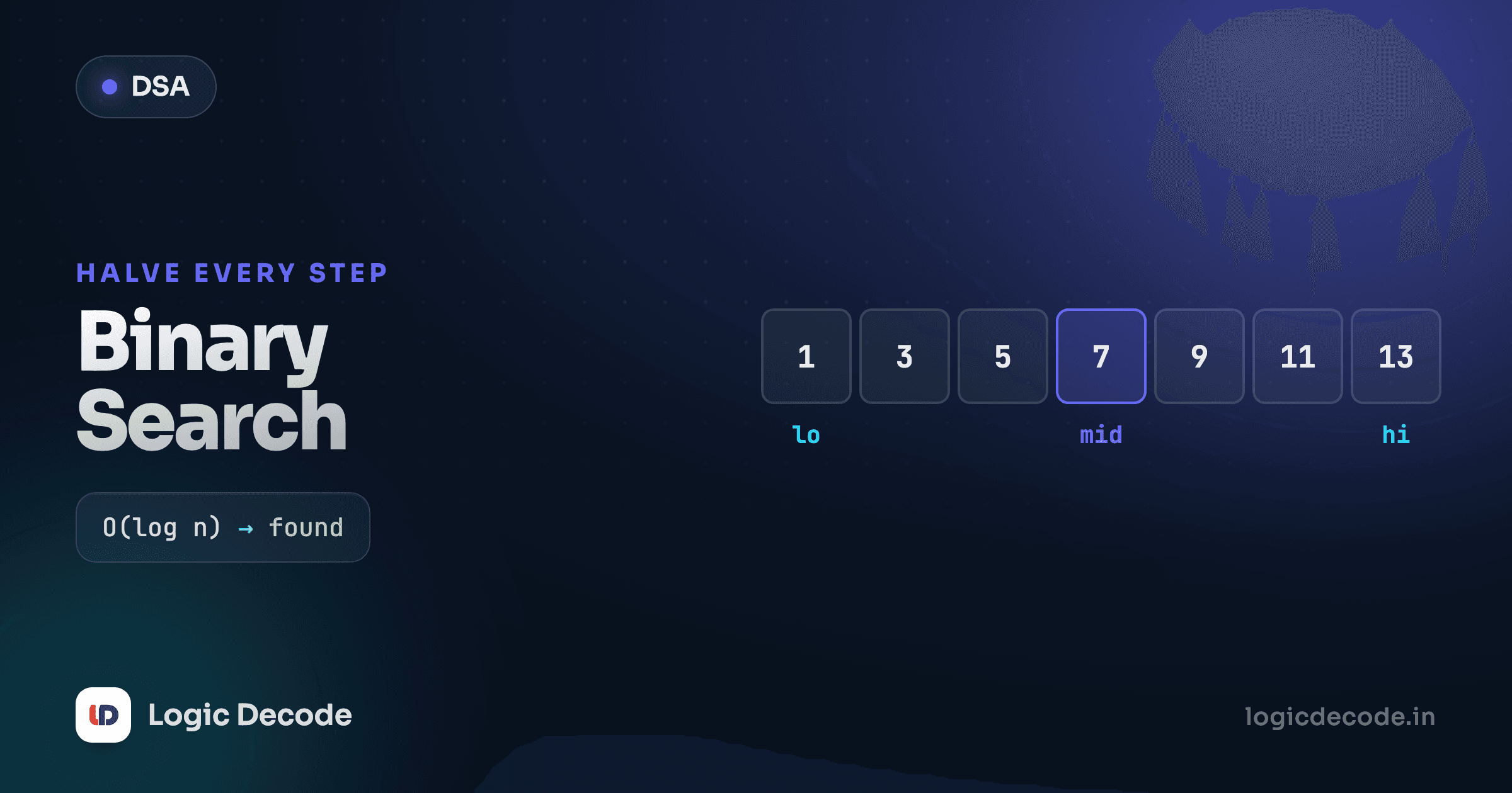
Binary search keeps a window over the part of the array that could still contain the target, marked by two indices: lo (the left edge) and hi (the right edge). Each step looks at the middle of that window:

• Compute mid = (lo + hi) // 2.
• If arr[mid] equals the target, you're done.
• If arr[mid] is too small, the answer must be to the right, so move lo to mid + 1.
• If arr[mid] is too big, the answer is to the left, so move hi to mid - 1.

Every comparison deletes half of what's left. The window shrinks 10 → 5 → 2 → 1 instead of 10 → 9 → 8.

Step through it below. Watch lo, mid, and hi jump as the window collapses around the target. The array is sorted ascending, which is the whole reason this works:

Trace what happened. The first mid lands near the middle of ten items. The target 23 is bigger, so lo leaps right and the left half is gone for good. A couple more splits and mid sits exactly on 23. You never looked at most of the array, and you never had to.

Write it once, run it

Here's the iterative version. It returns the index where the target lives, or -1 when the value isn't there. The loop condition lo <= hi is doing real work: the moment lo passes hi, the window is empty and the search has failed. Run it and edit the lookups:

Notice 100 returns -1. The window kept shrinking until lo overtook hi, the loop ended, and the function reported "not here." That clean failure case is as important as the success one. If you want a refresher on how while loops keep running until their condition breaks, the Python loops lesson covers it.

The catch that bites everyone

The speed is free only if the array is already sorted. Run binary search on unsorted data and it doesn't crash. It just lies, confidently returning wrong answers or -1 for values that are right there. The "smaller, so go right" logic assumes order, and without it every decision is a coin flip.

So binary search isn't a drop-in replacement for "find this value." It's a tool for sorted collections. Sometimes you sort once and search many times (worth it). Sometimes the data arrives sorted already, like a database index. Either way, the precondition is the price of admission.

What you've got

Binary search trades a one-time requirement (keep it sorted) for a massive speedup (O(log n) instead of O(n)). Track a window with lo and hi, check the middle, throw away the half that can't contain the answer, and repeat until you find the target or the window empties. That same divide-and-halve idea shows up again later when we build trees that stay sorted by design.

Next: Stacks and Queues — two of the simplest data structures, and the rules (LIFO and FIFO) that decide what comes out next.